
Breaking Down Momentum Strategies
Important ideas behind one of the most popular trading strategies


Introduction
By now I think it is safe to assume that everyone has heard enough about pairs trading so this article will take a break and look at one of the best strategies to start with - Momentum. Momentum is easy to do simply and hard to do amazingly. This makes it a great starting point as it is hard to fail with, but there is plenty of room to improve it.
This article will follow the same tune as the previous pairs trading guide where I share some knowledge I’ve gathered along the way on the best ways to implement momentum strategies / what to consider.
Index
Introduction
Index
Time Series vs Cross-Sectional
Beta Adjustment
Volatility Targeting
Regime Dependent Performance
Information Discreteness
Unexpected Volume Changes
Turnover Reduction & Portfolio Optimization
Continuous Features
PSD Momentum
Ensemble Ensemble Ensemble
Long-Term Momentum as a Factor
Backtest Duration Trickery
Conclusion
Time Series vs. Cross-Sectional
This will take many names (Relative vs. Absolute) (Momentum v.s Trend Following) but in general, the difference between time-series momentum and cross-sectional is that time-series momentum only uses the time series of each asset in isolation whereas cross-sectional is a relative measure of momentum.
A simple time-series momentum strategy could just be moving average crossover based, with a trailing stop-loss (since in this case losing money means no more edge so we can do this, in other cases stop-losses can create issues).
Our cross-sectional (relative) momentum strategy could be ranking our assets on their % price change, and then longing the top 10% and shorting the bottom 10%. As we will see in the next section this is a bad implementation.
Many practitioners like to argue over which one of these is the best approach, but there isn’t much in it between them and it is most likely that the optimal strategy is just an equally weighted ensemble of both relative & absolute momentum.
Beta Adjustment
One important thing to consider is the beta of each asset and how that plays into your momentum. If you are using relative momentum you will need to adjust each asset so it is a fair comparison and if you are using absolute momentum you may need to adjust your thresholds and parameters.
Let’s take the example of relative momentum. We can divide it into 2 market scenarios, a bull market, and a bear market. In a bull market, what happens?
Well, if the S&P500 goes up 1%, our largest % increase assets should just be the ones with the largest beta if we ignore momentum effects, and vice versa our lowest % change assets will be the ones with negative or small betas. This means we end up with a portfolio that is long beta in a bull market since most moves are positive.
If we now shift our attention to a bear market, what do we see? Well, we see the opposite, in a bear market the largest winners will be our assets with a negative beta or those with small betas, and our largest losers will be those with the largest beta.
See what just happened? We took a trade that was meant to be a momentum trade and ended up trading the beta factor. This is definitely not what we want, especially when we consider that the beta factor exposure isn’t even consistent - we are switching our exposure based on regime and it adds tons of extra noise.
The beta factor is a heavily debated factor and was shown in the equities market to be a linear combination of the profitability and conservative investment factors, but whilst this is a (maybe) factor (even if it isn’t orthogonal / is just a linear combination of others) we likely won’t get anywhere with it because we keep switching our bet on beta based on the market.
The fix is quite an easy one, we just adjust each asset for its beta. Simple as that. Now we know we aren’t trading beta / adding lots of noise to our equity curve. If an asset had a 10% return and a beta of 2, we just adjust it so that it had a 5% return (10 / 2).
Continuing the discussion of adjusting for beta, it is good practice to filter out the top decile assets by beta. This is a rule that holds true for many other alphas. Even when ignoring the additional turnover high beta assets tend to introduce, they still underperform on average and increase the portfolio risk unnecessarily.
Volatility Targetting
With volatility targeting we adjust our position sizing with the aim of keeping the portfolio volatility at some target level.
This ties into a few different objectives, namely:
Improving Sharpe ratio
Reducing turnover
Adjusting for recent volatility
Going down our list, we can start with the objective of improving the Sharpe ratio. We want to try to keep the rough gradient of our PNL curve the same, and one way to do this is to decrease our sizing when the portfolio is very volatile and vice versa when it is less volatile. This is part of our portfolio optimization in general but helps to improve our Sharpe ratio and keep gains consistent.
We will touch on the next point more in a later section, but it is a well-documented fact that the volatility of portfolio constituents is strongly tied to the turnover of the portfolio. If we go beyond adjusting for volatility and instead penalize for it, we can reduce turnover by making our portfolio constituents less volatile. There is also research indicating that regardless of turnover these lower volatility assets will perform better. We will touch on this point when discussing the role of news in momentum.
Finally, beta may only capture the long-term relationships to index moves and an asset that has had very high recent volatility due to some news/change in fundamentals may not have been properly accounted for. Strategies can use beta and volatility as an ensemble for best results. We want to penalize for volatility anyways, so adjusting for both is a smart move (how much we adjust for each is a parameter to optimize).
Regime Dependent Performance
It is a well-documented effect that momentum portfolios perform poorly during bear markets. This is an effect that is seen even when momentum is done properly and is not a result of portfolios capturing the beta factor, then switching long/short the factor based on a bull/ bear market (as discussed earlier).
Below is an extract from a paper showing this regime dependence:
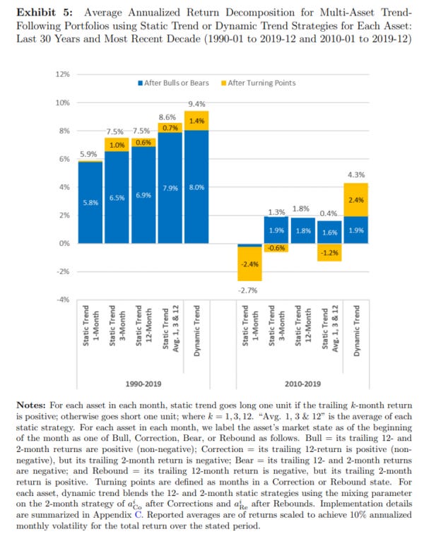
Momentum strategies suffer from a highly negative skew and are prone to sudden crashes, one severe example is that of 2008 where we saw < -90% drawdowns for equity momentum. At the same time, we also saw CTAs have an amazing year running momentum strategies in commodity markets. Diversification is always the best approach with momentum.
Whilst we cannot remove drawdown periods, we can attempt to avoid them. One of the best ways to do this is to use a regime classification filter to decide whether to trade or stay flat. Some approaches even suggest that the strategy should get take the inverse trade during these periods. This helps to improve performance significantly. An example of a simple filter is using the 1-year % change. If positive trade as normal, if negative stop trading or take the inverse.
This makes sense because momentum is effectively a bet on positively autocorrelated returns taking hold. If we see mean-reversion (negative autocorrelation) then we shouldn’t be running momentum. Bull markets are known for being positive autocorrelation regimes, whereas bear markets are known for being negative autocorrelation regimes. Bear markets are referred to as “choppy” which turns out to be trader speak for “mean-reversion friendly”. Thus, we want to flip to trading mean-reversion in bear markets where this takes hold, hence why we reverse our signals. I would argue that turning off the strategy and turning on a dedicated mean-reversion strategy would be a bit more optimal though.
For markets where cycles happen faster like cryptocurrencies, this filter should have a shorter period as bear/bull markets last for shorter durations. 90 days is usually my go-to but readers are free to experiment.
Information Discreteness
Momentum is a sustained increase or decrease in prices that we expect to continue. Therefore, we should filter out assets that have had large spikes up or down which are the main driver of their % change in price. We use information discreteness to capture how evenly distributed the changes in price are.
We define information discreteness (ID) below:
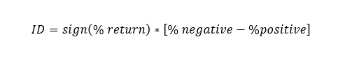
It is effectively the direction of overall returns multiplied by the % of positive samples - the % of negative samples. For a strategy that uses daily bars, this would be the % of days that were negative minus the % of days positive.
This lets us avoid news-driven price changes which have a much larger tendency to revert and of course, there is no expectation that we will see continued movement in price as the change was driven by the news. More on this in the PSD Momentum section.
Unexpected Volume Changes
We can further improve our momentum strategy by incorporating volume data. To normalize this data we can take the z-score of the dollar volume on an asset. Momentum tends to be far stronger when it is not driven by news and instead a result of flow.
Thus, we want to focus on assets that do not have an unexpectedly high volume, this is a sign that the move was likely a result of news. We are able to filter a lot of this out by using information discreteness, but in general, we do not want to enter into crowded trades so identifying momentum trades with the help of volume can help our performance.
I’d recommend winsorising the z-score / constructing your model in such a way that a z-score of 5 won’t cause some massive over/under allocation. You may also want to use a rolling period to sample volume over to reduce noise.
Readers can develop this idea further, potentially adjusting each day’s % return by its volume so that we penalize news-driven moves (which typically have high volume).
Many people like to classify momentum as an under or overreaction to information, but the best form of momentum has no new information at all. This is entirely behaviourally driven and is the ideal momentum to capture.
When the momentum/price change is driven by news we tend to see it as an overreaction, but this is a point we will explore more in the section on PSD momentum which behaves a little differently.
Lets classify momentum into two camps:
reaction to new information
behaviourally driven
For longer-term momentum, we want to exclusively capture #2. The section on PSD momentum will dig into how short-term momentum can be traded (which focuses heavily on information/market shock-driven momentum).
Turnover Reduction & Portfolio Optimization
We have discussed a few ways to decrease turnover using heuristic methods like penalising for volatility, but more advanced models can determine the optimal time to turnover the portfolio. It is common to use ranking-based methodologies where the top/bottom xx% of assets are longed/shorted.
Whilst this is a very quick way to do things, it is not the optimal way to do things, especially over the long run. If our current portfolio has an expected value of 8 bps and it will cost us 3 bps to replace it with the new top/bottom rankings, then we need to see an increase of (at minimum) 3 bps for this to be a good decision.
If we are just blindly using rankings then there is not even an estimate for the expected value of our portfolio so we would just switch our portfolio at rebalance time regardless of whether this decision makes sense. A dirty way to optimize turnover is to optimize the timing between rebalances, but this is also not a great idea for a proper implementation.
Thus, we need to estimate the EV of our portfolio. We can do this pretty easily with a trusty linear regression. This gets us an estimate for the expected value of each position. We can then use this information to only turnover the portfolio when it makes sense.
Mean-variance optimization (MVO) can also help us improve our Sharpe ratio, but it is not very robust to estimation errors so implementations like EPO (Enhanced Portfolio Optimization - Lasse Heje Pedersen, Abhilash Babu, and Ari Levine (2021)) help us avoid this issue and get a portfolio that optimizes our Sharpe ratio in a robust manner.
Going further than this we can use convex portfolio optimization models to include turnover costs in our portfolio construction process. Papers on this are referenced at the end.
Portfolio optimization models that account for turnover dig into some pretty complex math so it is certainly a fair bit of effort to build, but once implemented this model can be reused for many alphas in the future.
It is best to keep it simple when building portfolio optimization models so stick to the Boyd and Pederson papers and avoid the complicated models by grad students that typically perform worse out of sample despite being “theoretically” better.
The aim is to create a robust portfolio optimisation model which accounts for transaction costs.
Continuous Features
Now that we have a framework that allows us to decide whether or not to rebalance, our models can make use of continuous features without creating tons of turnover. Continuous features are simply features that do not depend on the granularity of the data itself and can thus be calculated continuously.
An example would be using a 30-day moving average instead of a 30-period moving average on daily data. Even if you were using tick data you would be able to calculate this 30-day moving average upon receiving new data. Whereas, if we were using a 30-period moving average on daily data we would need to wait for this data to have accumulated to form a 1-day bar.
Normally, we would end up with huge turnover if we used continuous features and evaluated our portfolio on every new piece of data, but with the use of turnover/portfolio optimization, we can now avoid this excessive turnover. The model will rebalance as soon as it is optimal. Ranking based methods lack the ability to determine if a rebalance is optimal and will likely turnover (partially) on almost every new piece of data. You can now use 5-minute bars, 15-minute bars, or whatever granularity you prefer despite working with alphas that on average rebalance once a day. Anything more granular than minute bars might be a bit unnecessary.
One issue we may run into with our data is the bid/ask bounce. As the asset trades between the bid and the ask price, the trade price will swap depending on whether the last order was a buy/sell and thus whether it hit the bid or the ask. This causes issues because our bars use the last trade price over the period to create the close price shown. If the close price is based on a buy in one bar, and then in the next bar it is based on a sell, the price will have leaped by an amount equal to the spread even if the midprice (fair value) stayed flat.
To avoid this issue, we can form our bars using the last midprice of the period. This common data error is incredibly under-known but plagues academic papers. There is a mountain of literature that references the short-term momentum reversal effect, but it was all an error. The effect is only present in small-cap assets, precisely the assets that would have wide spreads, and where the bid-ask bounce would create noticeable mean-reversion in the data (despite being fake). This effect goes away for all assets once you use metrics for fair value (midprice) instead of the last trade price.
PSD Momentum
PSD (Post-Shock Drift) Momentum is the momentum we tend to see after a shock hits the market. The most well-known of these is post-earnings announcement drift (PEAD) where an asset will tend to continue to drift in the direction of the initial move after the announcement of earnings that were surprising (significantly different from what the market had priced in).
This is not exclusive to earnings. Many announcements can be surprising even if there was no forecast for it in the first place. Any news which provides significant new information and thus causes a shock to the price can behave like this.
The effect has decayed significantly and there is no longer any profitability from trading these events without filtering. Especially for earnings releases it is almost entirely below transaction costs. Once a large shock has hit the market spreads will be incredibly high and your transaction costs will match so it isn’t an easy trade.
What we typically see is a large and sudden move as the market incorporates the information. This part is in the realm of HFT and is a whole other topic. Then we typically see a reversal as the market initially has overreacted to the news. After the reversal we often see PSD effects take hold.
In what scenarios do we typically see PSD take hold? and when is the initial overreaction the greatest (resulting in the largest reversal)? Well, these questions both share the same answer - when degens act like degens. If the shock is a piece of news that retail is expected to trade on heavily, perhaps a rumour makes them sell their assets, then we will see these sorts of effects in our data at a potentially profitable level.
For things like GDP announcements where retail isn’t in panic mode / isn’t taking YOLOs on it like the gamblers retail traders are, we do not see this effect. Reversals are barely pronounced and there is no significant momentum continuation at all.
I won’t dive too much into this effect and it can become very complicated to capture as you deal with the high spreads around these events and thus will want to use limit orders to trade. This isn’t exactly easy when there is a very short timeframe to enter this trade and the price will keep changing, forcing you to move up your limit order and chase the price as it gets away.
Identifying when uninformed flow will create PSD and the tricky issue of efficient execution both are topics I will leave to the reader to explore themselves.
Ensemble Ensemble Ensemble
This is one of the most important ideas for momentum strategies. The best model is the average of all models across all markets. Now, we should still make sure to do proper adjustments so we are actually capturing profitable momentum effects, but the question of whether to run Absolute vs. Relative momentum or what timeframe or what asset class are all best answered by our rule of always ensembling.
Running both absolute and relative momentum should create a better portfolio than either one alone. One might be slightly better than the other, and this may vary depending on the timeframe/ asset class / many other variables, but the combination of them will perform better than either of them on their own (on average).
Sometimes one version might get lucky and do better than the ensemble, but over the long run, it is pretty clear that the ensemble wins. This applies to timeframes as well. There are multi-period portfolio optimization models that can help with rebalancing portfolios constructed from alphas across different horizons.
CTAs are in the business of diversification. Whilst they may run other strategies, their bread and butter is momentum. This is something they apply to every market on the planet, thousands of futures, thousands of stocks, and much more all to improve their Sharpe ratio through diversification.
Long-Term Momentum as a Factor
I’ve discussed many ways to improve the performance of a momentum strategy, but for anything that isn’t intraday, you will not see stellar performance because longer-term (roughly anything holding for longer than a week) momentum behaves like a factor.
Momentum is a crowded trade and tons of people are doing it well. In some markets, it is the case that the best momentum model is actually the most popular - this is a lot more relevant for commodities than for equities. There is not going to be some new feature that allows you to make 3+ Sharpe. You can realistically get between 1.5 - 2.0 Sharpe by trading everything on the planet / diversifying tons, but going beyond that is hard without trading lower timeframes.
For PSD momentum you could easily hit massive Sharpe ratios but you are also dealing with low capacity due to liquidity evaporating around market shocks, have a MUCH harder time getting a strategy profitable, and only might have to hold risk for say 15 minutes until the momentum dies off. The most profitable strategies are hard!
Momentum behaving a bit like a factor is what makes it so easy for beginners. Even the simplest model can perform reasonably well. After improvements, we can definitely see index outperformance, but it won’t be RenTech levels, that’s for sure.
We already mentioned the large drawdowns that momentum strategies took during 2008, this was a clear example of overcrowding gone wrong. Diversification and researching simple methods to avoid crowded/unprofitable momentum trades are a large component of what will give you that outperformance. However, at the end of the day you are still capturing the same effect. There is only so much money on the table - you are just giving away less of it by making fewer mistakes and getting a smoother curve through diversification.
Backtest Duration Trickery
Many papers will only use the last 10 years for their momentum study, but that is very misleading. Not including 2008 as well as other momentum crashes is an easy way to make a strategy look a lot better than it really is by fitting to the current regime.
Good papers should test over multiple decades, some even look at centuries, this is important for long-term momentum as we want to use all the data we have. Especially in modern times, all assets have become so correlated that we cannot rely on a recent period alone. Even if we use many markets. Momentum evolves over time, ensure your strategy is robust across regimes / not just accidentally capturing the rise of tech stocks over the recent period through some modification that tends to favor them.
Conclusion
There’s a very long list of things I haven’t covered here and the literature on this subject is truly massive. I’ve done my best to at least show a few ideas that I think are important for doing momentum the right way, but a real deep dive through the resources out there is necessary to build an understanding.
Momentum is by far one of the best, if not the best, strategy to start with because you get to see results even when you are still learning. Intraday strategies - not so much. Profitability with momentum is easy after a few tries and some reading, whereas intraday strategies can take years of learning and experimenting before anything profitable is produced. It’s a great confidence booster to see that every strategy doesn’t fail (which tbh would otherwise be the case for a while starting out with intraday strategies).
Resources
Here I’ll give an informal list of resources to dig through for readers looking to dive deep into the world of momentum & trend following.
Read all the research articles in the archive on Alpha Architect. (The photo extract used in the regime dependence section is from a paper in one of the Alpha Architect articles)
https://alphaarchitect.com/research-category-list/
Read all the momentum / trend following articles on the Newfound Research blog.
https://blog.thinknewfound.com/
For portfolio optimisation:
Read Lasse Heje Pedersen’s paper on enhanced portfolio optimisation. He’s also got some amazing papers on momentum.
Stephen Boyd’s papers on convex portfolio optimisation as well as his textbook “convex optimisation” are brilliant. He’s got some great papers on convex optimisation with transaction costs.
Axioma Research Report Number 55, February 2015, Also available at http://www.axioma.com/downloads/MPOWithAlphaDecay.pdf
Anything Cliff Assness / AQR is a good read for momentum & trend following.
Some good macrocephalopod threads on the topic:
Robot James has some good content on his blog RobotWealth as well as his Twitter.
Corey Hoffstein’s podcast often has some great guests in the CTA / Momentum / Trend Following space.
Jack Vogel has a lot of good content out there (Alpha Architect being one) and has appeared on the above podcast. His textbook is a great read:
https://www.amazon.com/Quantitative-Momentum-Practitioners-Momentum-Based-Selection/dp/111923719X