
Professional Options Market Making & Taking [CODE INCLUDED]
How Optiver, IMC, and the rest of the pros decide how much an option is worth

Introduction
It’s been a busy few months for me, as I’ve started a new role a few months back in the world of linear instruments I’ve decided to write an article regarding some of my previous experience in options and how fair values are fitted as well as profited from.
When it comes down to it, the core money maker for making and taking remains roughly the same. Sure, you have maker models which don’t rely on vol curves (although they’re extremely simple to say the least) and there’s taker strategies that don’t do this, but by and large this is the most popular way of trading options at large institutions.
For a rough overview of how this article will be structured, we will first start with explaining how to fit some basic SSVI and SVI models. Then we’ll move on to working with the Wing model. Then we’ll explore a taker strategy where we exploit differences between the market fit vol curve and our values. We will also talk about how market makers fit their parameters that they then end up quoting around. In general, this is an options market making 101 guide for the pricing side of things.
This article will work with 2 models. The Orc Wing model which was a model used by Optiver as well as a range of other firms well over a decade ago, as well as SSVI (Stochastic Skew Volatility Inspired) which is publicly available in the literature. In modern times, Vola Dynamics is the choice model for most firms, if not an in-house proprietary solution. I’ve used Vola before but I can’t afford the $25,000-30,000 price tag per month or at least not until many many more people subscribe to this blog just for personal use and I’d have been fired if I used it to write an article at work so we’ll stick to slightly behind the leading edge.
We will be fitting cryptocurrency markets today which probably could use a C9 (9-parameter) curve as it isn’t exactly super advanced and there aren’t things like VIX options which can actually get you picked off on the tails if you were quoting something like SPY options (in which case you would be in the high teens, maybe even 20s).
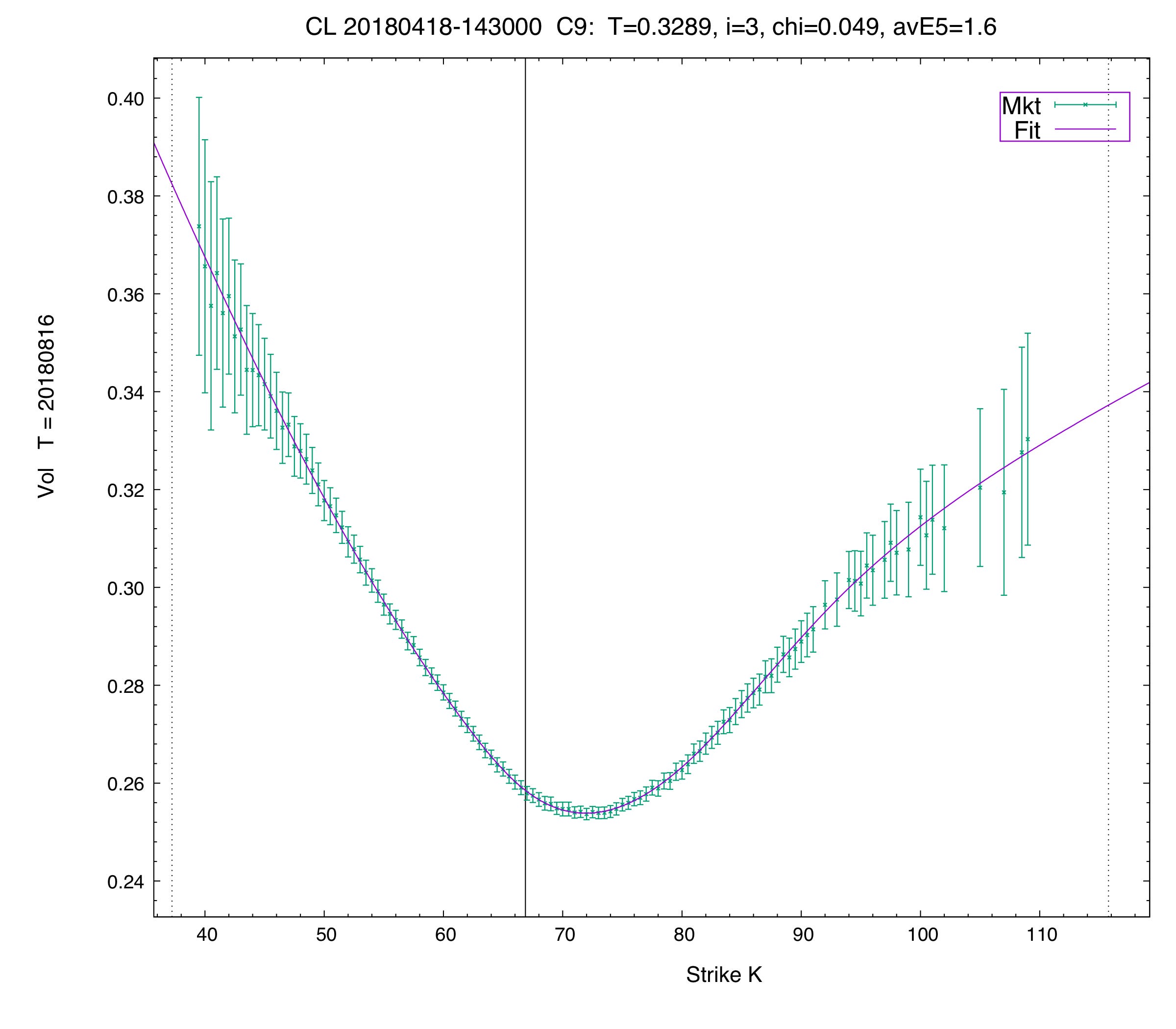
Above is what one of these looks like. Sadly, C9 curves are from Vola Dynamics so we will be using a 6 parameter model with the Orc model and an even more simplified model with only 3 parameters under the SSVI model. The reason I bring it up of course is to emphasize that unlike equity options, the markets for cryptocurrencies don’t require as complex a model and your time is best spent on figuring out other types of dynamics / strategy optimizations outside of the vol curve - which I won’t delve into now. SSVI is probably a bit too simple, but we’ll get away with it.
In all honesty, even if you were quoting around the Orc Wing model you’d probably be able to do quite well if your parameters had been fit properly (although if you have the opex to spend, get Vola still) in cryptocurrency markets whereas I would reserve the SSVI model for taking only whereas Orc is more capable of both. In equities, you’ll need Vola but that's a whole new ballpark
Index
Introduction
What’s a Vol Curve?
How to fit an SVI model so that it is arbitrage-free
Options Data Wrangling
Fitting SSVI parameters to the market
Patterns in SSVI models and exploiting them
When SSVI isn’t enough (it rarely is enough)
How to trade parameters themselves
Maker
Taker
Appendix: Orc Wing Model Code
What’s a Vol Curve?
Starting with a more proper explanation, a vol curve, like an SSVI curve, is basically a smooth function that maps the strike prices (or moneyness) of options to their implied volatilities in a way that looks realistic and consistent with market data. Think of it this way: for different options on the same underlying asset but with different strike prices, the implied volatility can vary—forming what’s called a “smile” or “skew.” An SSVI curve is one mathematically elegant method to fit (or interpolate) these implied volatility smiles so that they move in a plausible way over time and across strikes, so that traders (or risk managers, really whoever is using it at these prop firms) to price options consistently.
Really, a volatility curve is a generalization across all of the different options prices so we can reduce the dimensionality of what is a very high dimensionality asset class.
If I get filled on an option with X delta, Y gamma, etc etc, do I really want to have to fit a parameter for every single option I am quoting as to how this should change my pricing? And even if I do have that what if the delta or gamma of that option changes - how do those parameters even change? The point is, you just can’t do it the same way as it’s done in equities where you can simply have a pricing model for each different symbol and that’s it. Whether that’s the optimal model is a different question, but importantly - it can be done.
So what are these parameters and what do they represent for each of our models?
Let’s start first with the simpler model, SSVI. We have 3 main parameters: theta, rho, and phi. (k is just the strike in the below formula)
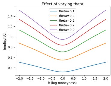
θ - Theta represents the total implied variance at-the-money. It’s basically the total level of the curve and doesn’t affect the shape of the curve, merely how high it is overall. Here’s what happens when we play around with it theta:
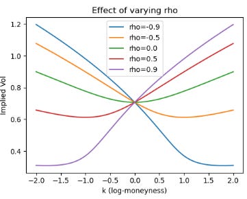
ρ - Rho represents the skew or the asymmetry of the curve. If we rotate the curve around we are saying put volatility is more expensive than calls or vice versa. It let’s us express whether we think large up or down moves are more likely. If we vary it we get this:
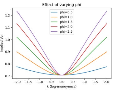
ϕ - Phi is the convexity of the curve, it changes how likely we think extreme moves are. Here’s what variations look like:
For those following along at home, here’s the code to run:
import numpy as np
import matplotlib.pyplot as plt

def ssvi_total_variance(k: float, theta: float, rho: float, phi: float) -> float:
    """
    Returns total implied variance w(k) under the SSVI parameterization:
    w(k) = (theta/2) * [ 1 + rho * phi * k + sqrt((phi*k + rho)**2 + 1 - rho**2) ]
    """
    return (theta / 2.0) * (
        1.0
        + rho * phi * k
        + np.sqrt((phi * k + rho) ** 2 + 1 - rho**2)
    )

# Create a range of log-moneyness points k
k_values = np.linspace(-2, 2, 200)

# -------------------------------
# 1) Vary theta
# -------------------------------
theta_list = [0.1, 0.3, 0.5, 0.7, 0.9]
rho_fixed = 0
phi_fixed = 2.00

plt.figure(figsize=(15, 4))

plt.subplot(1, 3, 1)
for theta in theta_list:
    w = ssvi_total_variance(k_values, theta, rho_fixed, phi_fixed)
    implied_vol = np.sqrt(w)  # T = 1 for simplicity
    plt.plot(k_values, implied_vol, label=f"theta={theta:.1f}")
plt.title("Effect of varying theta")
plt.xlabel("k (log-moneyness)")
plt.ylabel("Implied Vol")
plt.legend()

# -------------------------------
# 2) Vary rho
# -------------------------------
rho_list = [-0.9, -0.5, 0.0, 0.5, 0.9]
theta_fixed = 0.5
phi_fixed = 1.0

plt.subplot(1, 3, 2)
for rho in rho_list:
    w = ssvi_total_variance(k_values, theta_fixed, rho, phi_fixed)
    implied_vol = np.sqrt(w)
    plt.plot(k_values, implied_vol, label=f"rho={rho:.1f}")
plt.title("Effect of varying rho")
plt.xlabel("k (log-moneyness)")
plt.ylabel("Implied Vol")
plt.legend()

# -------------------------------
# 3) Vary phi
# -------------------------------
phi_list = [0.5, 1.0, 1.5, 2.0, 2.5]
theta_fixed = 0.5
rho_fixed = 0

plt.subplot(1, 3, 3)
for phi in phi_list:
    w = ssvi_total_variance(k_values, theta_fixed, rho_fixed, phi)
    implied_vol = np.sqrt(w)
    plt.plot(k_values, implied_vol, label=f"phi={phi:.1f}")
plt.title("Effect of varying phi")
plt.xlabel("k (log-moneyness)")
plt.ylabel("Implied Vol")
plt.legend()

plt.tight_layout()
plt.show()
How to fit an SVI model so that it is arbitrage-free
The formula I showed earlier is SSVI, it is the re-parameterization of SVI that enforces certain smoothness or arbitrage-free conditions more naturally (especially when done across expiries). In the below article, I showed some code for doing this with the raw SVI model which is generally a simpler model:
![Finding Fair Value [CODE INSIDE]](https://substackcdn.com/image/fetch/$s_!BX8O!,w_140,h_140,c_fill,f_webp,q_auto:good,fl_progressive:steep,g_auto/https%3A%2F%2Fsubstack-post-media.s3.amazonaws.com%2Fpublic%2Fimages%2F7ecb3472-4b44-4a63-9c04-91bc51c798e5_1035x801.png)
I won’t delve into the raw SVI model here since all the code and plots are in this article, but I will show how we fit the SSVI model in this chapter. There is also code for the Orc Wing model in that article, which I will actually toy about with in this article (later chapter).
Let’s first start with a slightly more complicated approach to things before leaving the SVI world for the SSVI and eventually Wing world. We will enforce no-arbitrage constraints using a penalty-based approach. We will enforce both butterfly and calendar arbitrage bounds for our options:
Let’s explain what these terms mean. First of all we have { a, b, σ, ρ, m }. These are rather simple and are the 5 parameters for the original SVI model (which can be read more about in the article mentioned earlier).
Next, we have w_raw( x; a, b, σ, ρ, m ) - this denotes the total implied variance at log-moneyness x. It’s basically just the model’s prediction for how much variance an option at strike x should have.
w_mkt is the market observed implied variance - our observed data.
∑n i=1(…)^2 - This is the least-squares term for optimization.
𝜏_i represents the time to expiry for the i-th maturity.
λ_cal represents a penalty weight for calendar arbitrage. If the model violates the arbitrage bound that variance should not decrease as time-to-expiration increases, a penalty is applied. The larger this value the more strictly we are enforcing the no-arbitrage bound.
max(0, w(x, 𝜏_i − 1) − w(x, 𝜏_i))^2 - this captures the calendar arbitrage violations. For a later maturity compared to an earlier maturity we want w(x, 𝜏_i − 1) <= w(x, 𝜏_i).
λ_fly represents the penalty weight for butterfly arbitrage similarly to how we set up the penalty for calendar arbitrage. It ensures the implied volatility curve remains convex enough to avoid negatively priced butterfly spreads. A larger value for this means a more strict enforcement of convexity.
Finally, g(x;a,b,σ,ρ,m) is out function which checks for butterfly arbitrage. If the SVI parameters lead to concavity or other violations, g becomes negative, and you pay a penalty max(0,−g(⋅))^2.
Okay… That’s enough math. Let’s put this into code, here’s our penalty functions: