
Semi-Definite Programming For SMRPs
Using SDP to create sparse mean-reverting portfolios (SMRPs) with variance constraints

Introduction
In the previous research article, we explored the use of Monte-Carlo Minimization (MCM) as a non-convex method for finding mean-reverting portfolios. Here we will use Semi-Definite Programming (SDP) to form mean-reverting portfolios with 2 major constraints. These are variance and sparsity.
SDP is a convex method which makes it a lot more robust compared to MCM. This means that it is far better suited to longer-term pairs trading portfolios as these prioritize forming robust portfolios whereas shorter-term portfolios are best built using models that can find more complex, but also shorter-lasting relationships.
We were able to produce a strategy with significant alpha in equities markets. Avid readers are welcome to solve the optimal spread trading problem in other ways and form their own strategies after building on this work.
Teasing results, we were able to generate significant alpha OOS using a robust methodology that makes overfitting far harder.
The Models
In addition to SDP, we will also be making use of Sparse Principal Component Analysis (SPCA) to enforce sparsity within our weight vector. Sparsity in this case means reducing the number of assets in our portfolio. We also want to add a minimum variance constraint to ensure that our portfolio is volatile enough to beat fees. To trade the spread we will use a set of Bollinger Bands. This is a very simple approach as our main focus is on portfolio generation methods.
The Data
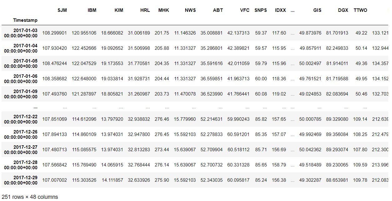
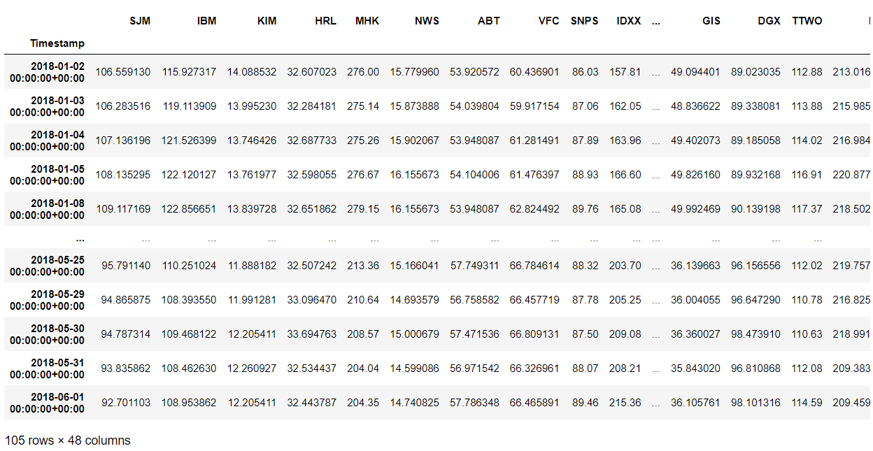
For this analysis, we shall use data from 2017-01-01 to 2018-01-01 for our training dataset, and 2018-01-01 to 2018-06-01 for our OOS dataset. This is equities data which comes from 50 randomly sampled S&P500 constituents.
Pre-Processing
We start by taking our data and arranging it into an array of column vectors containing daily close prices for our assets. Below is what our training (top image) and testing (bottom image) datasets look like:
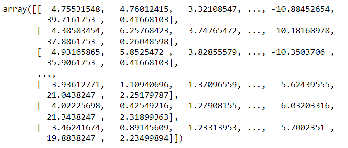
We then proceed to normalize our data. We first subtract the mean of each column, then we divide each column by the standard deviation of that column. We then get this Numpy array (for our training dataset)
VAR(1) Non-Sparse Optimization
We will give a quick example of how to optimize for a non-sparse portfolio using VAR(1) predictability as our optimization objective. There will also be no attempt to optimize for a minimum variance here.
We start by taking the autocovariance matrix of our normalized data using a lag of 0 and doing this again with a lag of 1. I’m sure some readers will have figured this out, but using a lag of 0 is just a normal covariance matrix.
We are effectively solving for the matrix x which minimizes our variance ratio, this is expressed as the below problem:
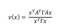
We know that minimizing this variance ratio is the same as finding the minimum generalized eigenvalue 𝜆 in the equation:
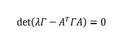
The portfolio that thus minimizes the variance ratio 𝑣(𝑥) is given by:
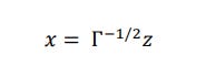
Where 𝑧 is the eigenvector that corresponds to the minimum eigenvalue of the matrix denoted:
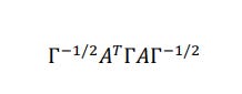
Rho is our covariance matrix, and A is the coefficients of our vector autoregressive model.
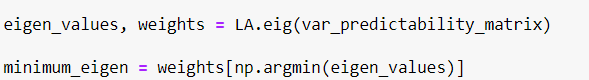
Expressing this as code we perform the below series of operations. cov_matrix is our covariance matrix (autocovariance matrix with lag 0) and autocov_matrix is our autocovariance matrix with lag 1.

We then take the eigenvalues of this matrix and then grab the eigenvector (our portfolio weights) corresponding to the minimum eigenvalue.
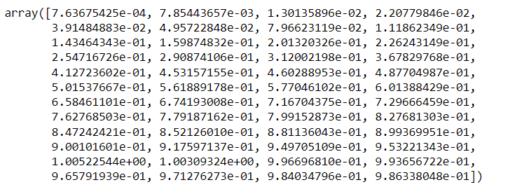
Our eigenvalues look like this:
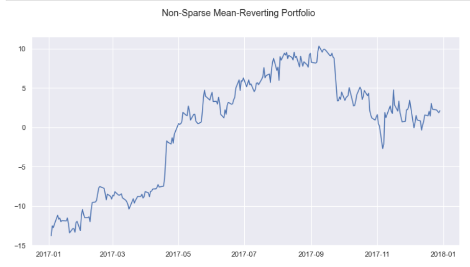
Taking the dot product of our previously mentioned normalized training dataset with our minimum_eigen variable (the weights) we get the portfolio below:
Semi-Definite Programming & SPCA
Now that we have generated our non-sparse portfolio without minimum variance constraints we will now create a portfolio that is both sparse and meets minimum variance constraints using Semi-Definite Programming and SPCA.
Giving a glimpse into our optimization problem:

This is all done using CVXPY which is quite an easy task so I won’t walk through this part too much. We use a matrix norm penalty which is equivalent to the alpha parameter of our SPCA to induce sparsity.
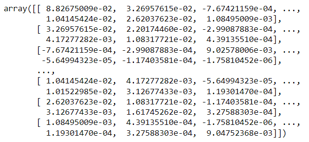
We get the target selection of eigenvectors given below from solving with SDP:
After we apply SPCA we get:
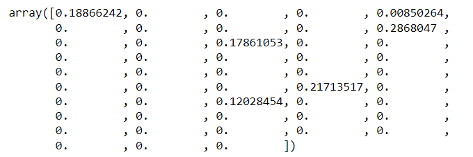
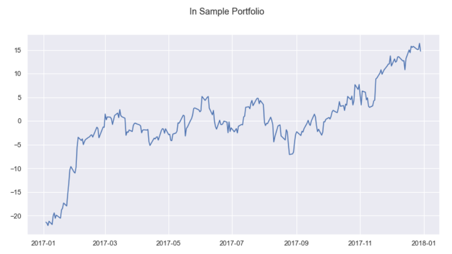
This array (which is our portfolio weights) can be used to generate the below portfolio:
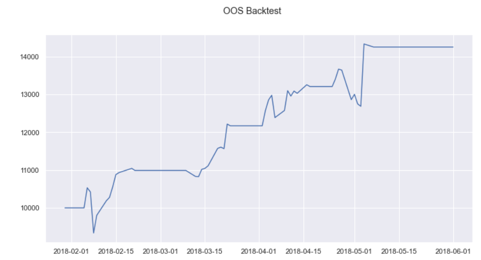
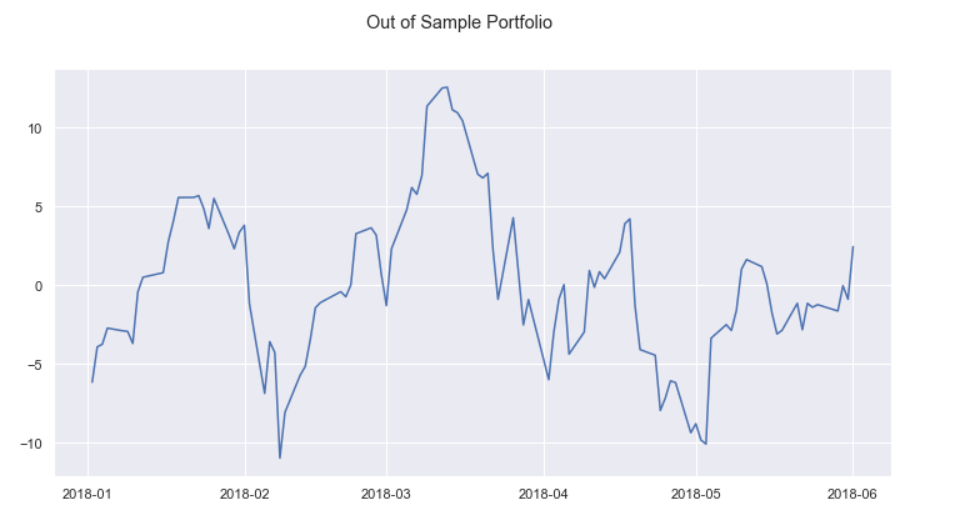
Applying these weights to our out of sample dataset we get:
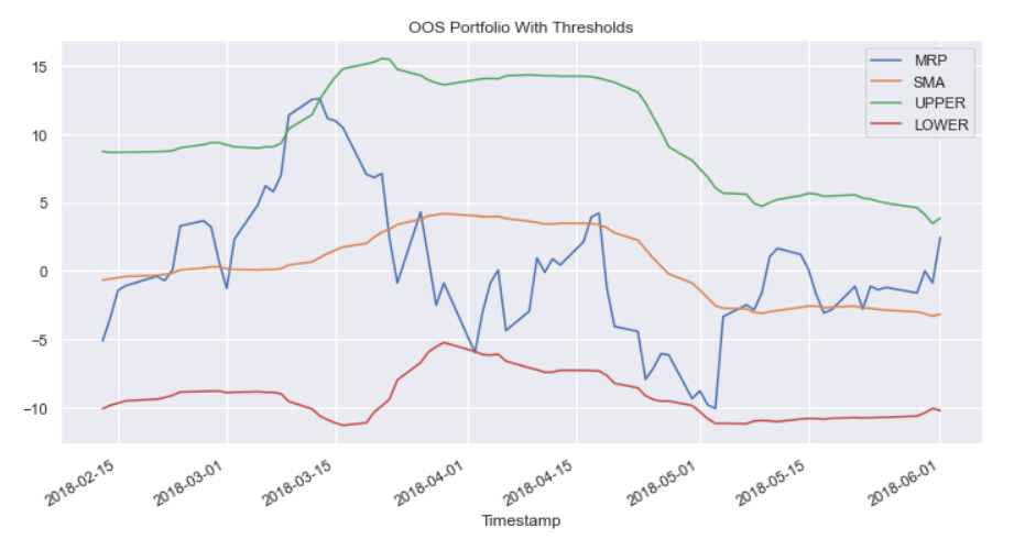
Trading The Spread
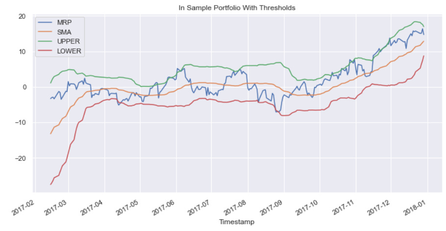
We will be applying a simple 20-period moving average as our rolling mean, with bands that are +/- 2SD (computed as a 20-period rolling standard deviation). This is just Bollinger Bands for the degens out there. It is far from the optimal way to do it, but trading the spread is not the focus of this article.
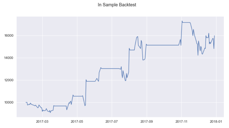
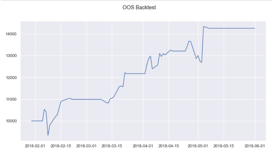
Doing this, our in-sample and OOS portfolios look like this:
Results
Trading these thresholds by getting short the spread if it is above the upper band, then exiting at the mean, AND getting long the spread if it is below the lower band, then exiting at the mean results in the below performance:
Conclusion
We were able to show that there is significant alpha in pairs trading still, but this does not come from outdated methods static thresholds, and ADF. We can further improve this performance by creating additional optimization metrics which can improve the volatility, trading costs, and mean-reversion characteristics of our portfolio.
Eager users may also want to explore my other articles on portfolio generation for pairs trading and may attempt to build on this using methods like pattern matching and stochastic control for more optimal pairs trading (these methods are only optimal for higher resolution data, they are too much / will suck for a longer-term portfolio like the one shown).
If you want further reading on this topic I’ve added some papers below.
Papers
BOX, G. E., and G. C. TIAO. “A Canonical Analysis of Multiple Time Series.” Biometrika, vol. 64, no. 2, 1977, pp. 355–365., https://doi.org/10.1093/biomet/64.2.355.
D'Aspremont, Alexandre. “Identifying Small Mean-Reverting Portfolios.” Quantitative Finance, vol. 11, no. 3, 2011, pp. 351–364., https://doi.org/10.1080/14697688.2010.481634.
Deadman, Edvin, et al. “Blocked Schur Algorithms for Computing the Matrix Square Root.” Applied Parallel and Scientific Computing, 2013, pp. 171–182., https://doi.org/10.1007/978-3-642-36803-5_12.
Fogarasi, Norbert, and Janos Levendovszky. “Sparse, Mean Reverting Portfolio Selection Using Simulated Annealing.” Algorithmic Finance, vol. 2, no. 3-4, 2013, pp. 197–211., https://doi.org/10.3233/af-13026.
Göncü, Ahmet, and Erdinç Akyıldırım. “Statistical Arbitrage with Pairs Trading.” International Review of Finance, vol. 16, no. 2, 2016, pp. 307–319., https://doi.org/10.1111/irfi.12074.